Lecture 2: Introduction, Linear Regression, Gradient Descent
Introduction
Welcome
Machine learning is used in algorithms that rank web-pages, recognizes people in photos, or even filters your spam. These algorithms try to mimic how the human brain works. Normally machines would do one specific task that was stated by the algorithm, but as the variety of tasks increase we realize the only way to catch up is to create such algorithms through which machines can teach themselves to do the task.
What is Machine Learning?
Ability to learn without explicitly being programmed (definition by Arthur Samuel). Extra reading: this and this.
A newer defnition by Tom Mitchell: a computer program is said to learn from experience E with respect to some task T and some performance measure P, if its performance on T, as measured by P, improves with experience E.
Example: playing checkers.
E = the experience of playing many games of checkers
T = the task of playing checkers.
P = the probability that the program will win the next game.
Machine learning algorithms are broadly classified into:
-
Supervised Learning
-
Unsupervised Learning
Other terms include: Reinforcement learning, recommender systems.
Supervised Learning
For housing price prediction, you collect data of the size of the house and the price. You then graph the data and you can either perform a linear regression to predict the prices of other houses or pass a quadratic line through the graph for the same. This is an example of supervised learning solved through regression (predict continuous values).
For classifying whether or not a tumor of size x is malignant or benign. This is a classification problem. To this problem you can add more features, and so if there were about infinite features to deal with it we use support vector machines and this.
Unsupervised Learning
We’re given a dataset that isn’t labeled, and not told what to do with it. So then, the algorithm must create clusters through a clustering algorithm. Unsupervised learning allows us to approach problems with little or no idea what our results should look like. We can derive structure from data where we don’t necessarily know the effect of the variables. We can derive this structure by clustering the data based on relationships among the variables in the data. With unsupervised learning there is no feedback based on the prediction results.
Like Google news clusters news stories together from thousands of news articles posted online. Other examples include: analyzing customer data and creating clusters for them, social network analysis, astronomical data analysis, organizing computing clusters.
Clustering: Take a collection of 1,000,000 different genes, and find a way to automatically group these genes into groups that are somehow similar or related by different variables, such as lifespan, location, roles, and so on.
Cocktail Party Problem
Non-clustering: The “Cocktail Party Algorithm”, allows you to find structure in a chaotic environment. (i.e. identifying individual voices and music from a mesh of sounds at a cocktail party).
To solve the cocktail party problem, we use ICA: Independent Component Analysis.
Basically separates the sounds coming from two different sources. This is done through just one line of code: \([W,s,v] = svd((repmat(sum(x. * x,1),size(x,1),1). * x) * x');\)
Model and Cost Function
Model Representation
Taking the housing price example, you are given m number of training examples, x is the input variable/features and y is the output variable/features. (x, y) refers to a single training example and \((x^{i}, y^{i})\) is the \(i^{th}\) training example.
h(hypothesis) is a function that maps from x to y. To represent h, \(h(x) = \theta_0 + \theta_1 x\) (linear or affine function) and if there are more inputs: \(h(x) = \theta_0 + \theta_1 x_1 + \theta_2 x_2 ... = \sum_{j=0}^{z} \theta_j * j\)
To establish notation for future use, we’ll use \(x^{(i)}\) to denote the “input” variables (living area in this example), also called input features, and \(y^{(i)}\) to denote the “output” or target variable that we are trying to predict (price). A pair \((x^{(i)} , y^{(i)} )\) is called a training example, and the dataset that we’ll be using to learn—a list of m training examples \({(x^{(i)} , y^{(i)} ); i = 1, . . . , m}\) —is called a training set. Note that the superscript “(i)” in the notation is simply an index into the training set, and has nothing to do with exponentiation. We will also use X to denote the space of input values, and Y to denote the space of output values. In this example, \(X = Y = ℝ\).
To describe the supervised learning problem slightly more formally, our goal is, given a training set, to learn a function \(h : X → Y\) so that h(x) is a “good” predictor for the corresponding value of y. For historical reasons, this function h is called a hypothesis.
When the target variable that we’re trying to predict is continuous, such as in our housing example, we call the learning problem a regression problem. When y can take on only a small number of discrete values (such as if, given the living area, we wanted to predict if a dwelling is a house or an apartment, say), we call it a classification problem.
Cost Function
| Size in \(feet^2\) \((x^2)\) | Price in $ in 1000’s (y) |
|---|---|
| 2104 | 460 |
| 1416 | 232 |
| 1534 | 315 |
| 852 | 178 |
| … | … |
for \(\theta_0 = 1.5\) and \(\theta_1 = 0\)
for \(\theta_0 = 0\) and \(\theta_1 = 0.5\)
for \(\theta_0 = 1\) and \(\theta_1 = 0.5\)
The idea is to select \(\theta_0\) and \(\theta_1\) so that \(h_\theta(x)\) is close to \(y\) for our training examples \((x, y)\). To do this we have to minimize this function: \(\sum_{i=1}^{m} (h_\theta(x^{(i)}-y^{(i)}))^2\) and to minimize the work you average it out by a factor of \(2m\) and use this: \(J(\theta_0, \theta_1) = \frac{1}{2m} (h_\theta(x^{(i)}-y^{(i)}))^2\).
Why is it mean-squared error and not to the power of 4 or something else?
We can measure the accuracy of our hypothesis function by using a cost function. This takes an average difference (actually a fancier version of an average) of all the results of the hypothesis with inputs from x’s and the actual output y’s. This function is otherwise called the “Squared error function”, or “Mean squared error”. The mean is halved as a convenience for the computation of the gradient descent, as the derivative term of the square function will cancel out the \(\frac{1}{2}\) term.
Cost Function Intuition
Hypothesis: \(h_\theta(x) = \theta_0 + \theta_1 x\)
Parameters: \(\theta_0, \theta_1 ...\)
m: number of training examples
n: number of features
x: inputs / features
\[x = \begin{bmatrix} x_0\\ x_1\\ x_2 \end{bmatrix}\]where, \(x_0\) is zero all the time \(x_1\) is size in feet \(x_2\) is number of bedrooms
\[\theta = \begin{bmatrix} \theta_0\\ \theta_1\\ \theta_2 \end{bmatrix}\]y: output / target variable
Cost Function: \(J(\theta_0, \theta_1) = \frac{1}{2m} (h_\theta(x^{(i)})-y^{(i)})^2\)
Goal: \(J(\theta_0, \theta_1)\)
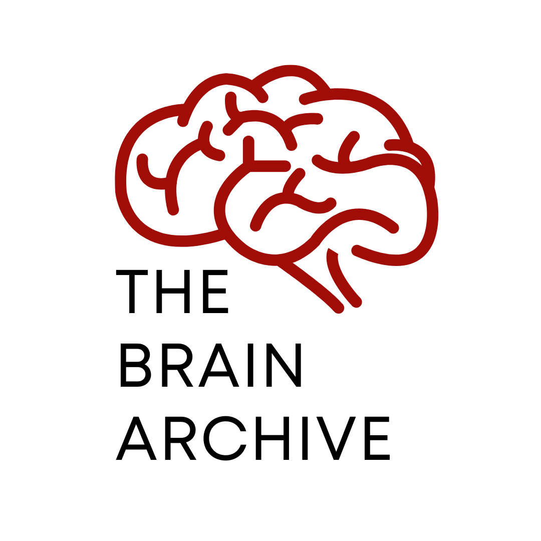
If we try to think of it in visual terms, our training data set is scattered on the x-y plane. We are trying to make a straight line (defined by \(h_\theta(x) = h(x)\) which passes through these scattered data points.
Our objective is to get the best possible line. The best possible line will be such so that the average squared vertical distances of the scattered points from the line will be the least. Ideally, the line should pass through all the points of our training data set. In such a case, the value of \(J(\theta_0, \theta_1)\) will be 0. The following example shows the ideal situation where we have a cost function of 0.
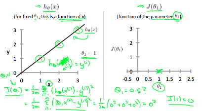
When \(\theta_1 = 1\), we get a slope of 1 which goes through every single data point in our model. Conversely, when \(\theta_1 = 0.5\), we see the vertical distance from our fit to the data points increase.
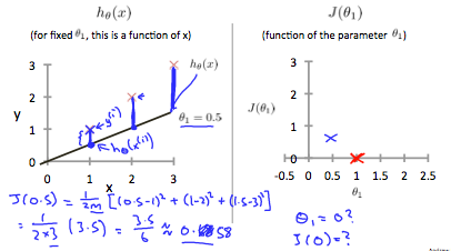
This increases our cost function to 0.58. Plotting several other points yields to the following graph:
Thus as a goal, we should try to minimize the cost function. In this case, \(\theta_1 = 1\) is our global minimum.
To embed plots on your jekyll blog try this, this and this.
Found this really neat blog here for better notes than mine.
Is it weird that in all my years of studying math, that somehow making a graph for a blog post no one shall read led to the enlightenement of how important math is?
Parameter Learning
Gradient Descent
Before any of this, watch the 3Blue1Brown video:
A cost function is a function that measures the performance of a machine learning model for a given data. It quantifies the error between the predicted values and the expected values (to a single number).
Depending on the problem Cost Function can be formed in many different ways. The purpose of Cost Function is to be either:
- Minimized: then returned value is usually called cost, loss or error. The goal is to find the values of model parameters for which Cost Function return as small number as possible.
- Maximized: then the value it yields is named a reward. The goal is to find values of model parameters for which returned number is as large as possible.
Gradient descent is an optimization algorithm used to find the parameters to minimize the cost function.
The cost function here is \(J(\theta) = \frac{1}{2m} (h_\theta(x^{(i)})-y^{(i)})^2\) and we need to minimise it. Keep changing \(\theta\) to reduce \(J(\theta)\)
\[\begin{eqnarray} J \left(\begin{pmatrix}\theta_0\\ \theta_1\end{pmatrix} \right) &=& \frac{1}{2m}\sum_{i=1}^{m} (h(x^{(i)})-y^{(i)})^2 \\ &=& \frac{1}{2m}\sum_{i=1}^{m} ((\theta_0 + \theta_1 x^{(i)})-y^{(i)})^2 \\ &=& \frac{1}{2m}(X\times\Theta-y)'\times (X\times\Theta-y) \end{eqnarray}\]To change \(\theta\) we say \(\theta_j := \theta_j - \alpha \frac{\partial J(\theta)}{\partial \theta_j}\) for \(j = 0, 1, 2, ...\) (here := is an assignment operator it’s like \(a = a + 1\) is wrong but \(a:= a + 1\) is correct).
\[\frac{\partial J(\theta)}{\partial \theta_j} = \frac{\partial}{\partial \theta_j} \frac{1}{2} (h_\theta(x) - y)^2\\=2 \frac{1}{2} (h_\theta(x) - y) \frac{\partial}{\partial \theta_j} (h_\theta(x) - y)\\=(h_\theta - y) \frac{\partial}{\partial \theta_j} (\theta_0 x_0 + \theta_1 x_1 + ... + \theta_d x_d - y)\\=(h_\theta - y) x_j\]So now we can say: \(\theta_j := \theta_j - \alpha(h_\theta(x)-y) x_j\)
\[\theta_j := \theta_j - \alpha\sum_{i=1}^{m} (h_\theta(x^{(i)}-y^{(i)}))x_j\]This is called batch gradient descent.
Stochastic gradient descent
repeat {
    for i = 1 to m {
        for j = 1 to d {
            theta_j := theta_j - alpha h_theta(x^{(i)}-y^{(i)}))x_j^(i)
        }
    }
}
Unlike batch gradient descent, stochastic never converges but runs fatser on large datasets.
mini-batch gradient descent.
Gradient Descent Intuition
Gradient Descent for Linear Regression
The math is pretty simple: learn the basic matric operations, transpose, inverse and multiplication.
\(tr(A) =\) Trace of Matrix A = sum of the diagonals
\[tr(A) = tr(A)^{T}\] \[f(A) = tr(AB)\\\nabla_{A} F(A) = B^{T}\] \[tr(AB) = tr(BA)\] \[tr(ABC) = tr(CAB)\] \[\nabla_{A} tr(AA^{T}C) = CA + C^{T}A\][watch again]