
Lecture 3: Locally Weighted & Logistic Regression
Okay so now instead of just straight lines, we’ll be dealing with curves and so the definition of \(h(x) = \theta_0 + \theta_1 x_1 + \theta_2 x_2 ...\) changes from this to something like a qudratic line \(h(x) = \theta_0 + \theta_1 x_1 + \theta_2 x_2^2\) and if we don’t want it to look like a parabola we could say \(h(x) = \theta_0 + \theta_1 x_1 + \theta_2 \sqrt[2]{x_2}\)
Now feature design algorithms help to decide whether x should be squared or rooted or should the log of x be taken so as to fit the function.
Locally Weighted Regression
What if the data isn’t fit well by just a straight line? How do you find the features then? We use locally weighted regression.
Parmetric lerning algorithms: Fit a fixed set of parameters \(\theta_i\) to the data.
Non-parametric learning algorithms: (locally weighted uses this) The amount of data/parameters you need to keep grows linearly with the size of data. (Not great if you have a large dataset becasue you need to keep all the data around loaded in the memory)
In linear regression: To evaluate the output at x, fit \(\theta\) to minimize the cost function \(J(\theta_0, \theta_1) = \frac{1}{2m} (y^{(i)}-\theta^{T}(x^{(i)}))^2\) and return \(\theta^{T}(x)\)
In a locally weighted regression you look at those value close to the value you want to predict and draw a line there.
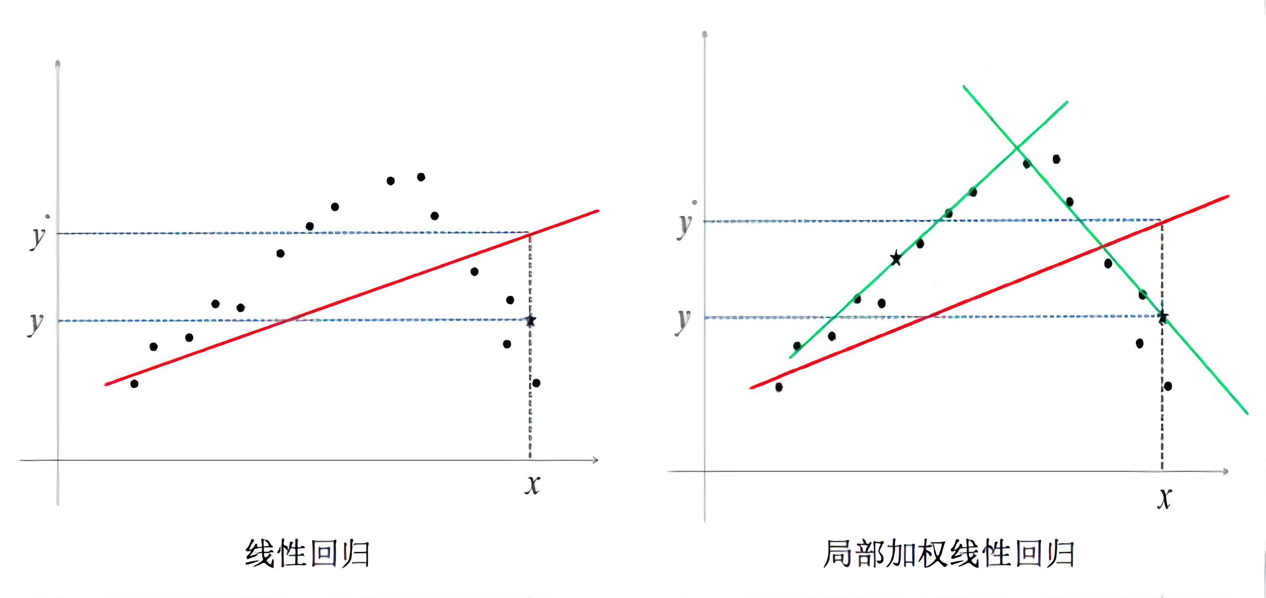
In locally weighted regression, fit \(\theta\) to minimize \(\sum_{i=1}^{m} w^{i} (y^{(i)}-\theta^{T}(x^{(i)}))^2\) where \(w^{i}\) is a “weight” function.
A default choice of \(w^{i}\) will be \(exp(\frac{-(x^{(i)}-x)^2}{2\tau^2})\) and if \(\mid x^{(i)}-x \mid\) is small then \(w^{(i)} \approx 1\) and if \(\mid x^{(i)}-x \mid\) is large then \(w^{(i)} \approx 0\). So now if the term that you predit is far away from an \(x^{(i)}\) then multiply the term with zero.
How do you choose the widh of the gaussain function? The parameter \(\tau\) is the bandwidth parameter that lets you decide on how big the neighbourhood of the value to be predicted should be. Depending on \(\tau\) we can choose a fatter or thinner bell shaped curve. The value of \(\tau\) has an influence on whether the data is underfitted or overfitted.
Probabilistic Interpretation
Why is the least square error taken? [24:00]
[53:55]
Now in the whether the tumor is malignant example, the probability of it being malignant is \(p(y=1 \mid x; \theta) = h_\theta(x)\) and of it not being malignant is \(p(y=0 \mid x; \theta) = 1 - h_\theta(x)\) and these two equations can be combined as: where \(y \in {0, 1}\), \(p(y \mid x; \theta) = (h_\theta(x))^y (1 - h_\theta(x))^{1-y}\)
And we come back to the exact same equation as we had in
[1:06:00]
Newton’s Method
Gadient descent is too slow because of the number of iterations it takes. Newton’s method takes more costlier iterations but the number decreases.
Starting from an initial point always draw a tangent and see where the tangent meets the x-axis such thta y = 0. Then if on that point x is not equal to 0 keep repeating the process.
It has quadratic convergence.