
Morlet Wavelets [Part 1]
Morlet Wavelets (Usage and Python Implementation)
We might lose data while converting the signals of EEG from the time to frequency domain. That’s a short-coming of static spectral analyses, and so to be able to extract frequency specific information over time we use wavelet convolution.
What’s a wavelet?
Yeah, there’s a bit of cheating, we can’t graph complex numbers in desmos and I’ll probably have to look into plotting these another way, but for now the only online substitute is visit this and type this: \(\cos (2\pi z)+z\sin (2\pi z)\) z(from Euler’s formula) and like all things complex, you must imagine yourself multiplying it with a gaussian and creating a morlet.
Euler’s formula for the basic waves \(e^{2\pi i \theta}\) is \(e^{2\pi i \theta} = cos(2\pi\theta) + i sin(2\pi\theta)\).
The Arctic Monkeys logo might be more mathematic than you think.
かわいいですね💮
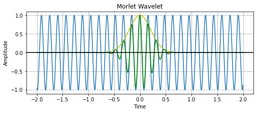
Requirements for a wavelet: it integrates to zero or the sum total is zero over time and it tapers to zero in the beginning and the end.
Wavelets provide temporal specificity when used as weighting functions for signals, as when these signals are convoluted(sliding dot product between the kernel and the section of signal it’s aligned with) with the kernel(in this case the morlet wavelet).
import math
import numpy as np
import matplotlib.pyplot as plt
plt.rcParams["figure.figsize"] = (8,3)
srate = 1000
# changed time from [-1,1] to [-2,2] to get a better guassian resolution
time = np.linspace(start = -2, stop = 2, num = 1000)
freq = 2 * np.pi
# using euler's to ceneter the sine at zero (it looks okay)
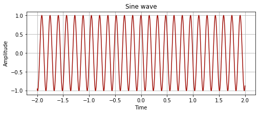
sine_wave = np.cos(2 * np.pi * freq * time) - 0.1 * np.sin(2 * np.pi * freq * time)
def plot_signal(x, y, title, x_label = "Time", y_label = "Amplitude", zoom = "no"):
    plt.plot(x, y, color = "#9F0D06")
    plt.title(title)
    plt.xlabel(x_label)
    plt.ylabel(y_label)
    plt.grid(True, which='both')
    # plt.axhline(y=0, color='k')
    if zoom == "yes":
        plt.margins(x=0, y=-0.001)
        plt.xlim(0,40)
    plt.show()
plot_signal(time, sine_wave, "Sine wave")
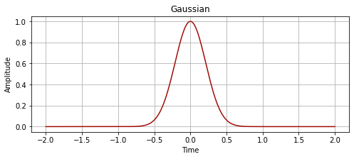
We want to create a guassian with a full width at half maximum (FWHM), where the FWHM is the width of a line shape at half of its maximum amplitude, as shown below:

# defining the gaussian
# full width at half maximum
fwhm = 0.5
gaussian = np.exp((-4 * np.log(2) * (time)**2) / (fwhm**2))
plot_signal(time, gaussian, "Gaussian")
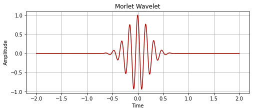
# element-wise multiplication of the sine and gaussian
morlet_wavelet = sine_wave * gaussian
plot_signal(time, morlet_wavelet, "Morlet Wavelet")
# looking at everything at once.
plt.plot(time, sine_wave)
plt.plot(time, gaussian, 'y')
plt.plot(time, morlet_wavelet, 'g')
plt.title('Morlet Wavelet')
plt.xlabel('Time')
plt.ylabel('Amplitude')
plt.grid(True, which='both')
plt.axhline(y=0, color='k')
plt.show()
pnts = time.shape[0]
mwX = 2 * abs(np.fft.fft(morlet_wavelet)/pnts)
hz = np.linspace(start = 0, stop = srate, num = pnts)
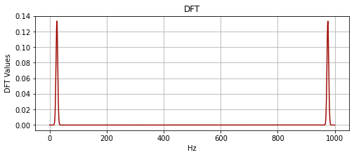
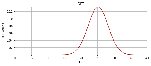
plot_signal(hz, mwX, "DFT", "Hz", "DFT Values")
plot_signal(hz, mwX, "DFT", "Hz", "DFT Values", "yes")
import pandas as pd

time_series = pd.read_csv("data.csv")
time_series_values = time_series["value"].to_numpy()
time_series_values = np.append(time_series_values, time_series_values)
time_series_values = np.append(time_series_values, time_series_values)
time_series_values = np.append(time_series_values, time_series_values)
time_series_time = np.linspace(start = 0, stop = 100, num = len(time_series_values))
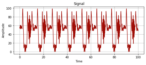
plot_signal(time_series_time, time_series_values, "Signal")
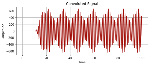
convoluted_signal = np.convolve(time_series_values, morlet_wavelet, 'full')
plot_signal(time_series_time, convoluted_signal[:len(time_series_time)], "Convoluted Signal")
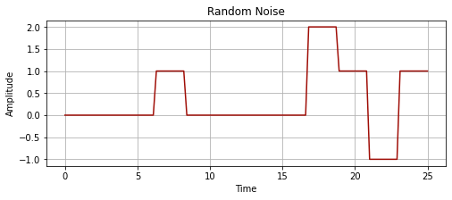
x1 = np.zeros(30)
x2 = np.ones(10)
x3 = np.zeros(40)
x4 = np.ones(10)*2
x5 = np.ones(10)*-1
time_series_values_2 = np.array([])

time_series_values_2 = np.append(time_series_values_2, x1)
time_series_values_2 = np.append(time_series_values_2, x2)
time_series_values_2 = np.append(time_series_values_2, x3)
time_series_values_2 = np.append(time_series_values_2, x4)
time_series_values_2 = np.append(time_series_values_2, x2)
time_series_values_2 = np.append(time_series_values_2, x5)
time_series_values_2 = np.append(time_series_values_2, x2)

time_series_time_2 = np.linspace(0, 25, len(time_series_values_2))

plot_signal(time_series_time_2, time_series_values_2, "Random Noise")
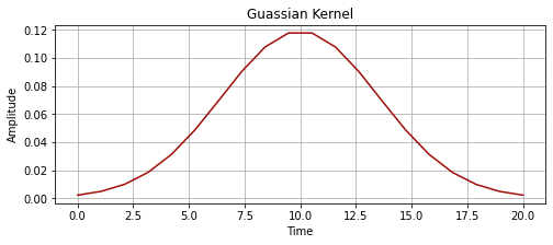
kernel_new = np.exp(-np.linspace(-2,2,20)**2)
kernel_new = kernel_new / np.sum(kernel_new)
# try these
# kernel_new = -1 * kernel_new
kernel_time = np.linspace(0, 20, 20)
plot_signal(kernel_time, kernel_new, "Guassian Kernel")
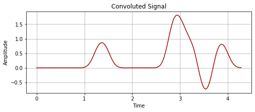
# smooths out the signal
convoluted_signal = np.convolve(time_series_values_2, kernel_new, 'full')
plot_signal(time_series_time[:len(convoluted_signal)], convoluted_signal, "Convoluted Signal")
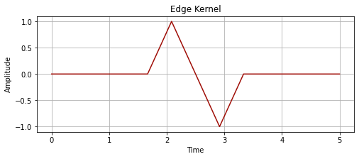
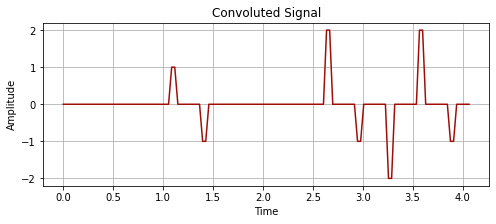
# let's try building the edge detecting kernel

kernel_edge = np.array([])
x6 = np.zeros(5)
x7 = np.ones(1)
x8 = np.zeros(1)
x9 = np.ones(1) * -1

kernel_edge = np.append(kernel_edge, x6)
kernel_edge = np.append(kernel_edge, x7)
kernel_edge = np.append(kernel_edge, x8)
kernel_edge = np.append(kernel_edge, x9)
kernel_edge = np.append(kernel_edge, x6)

kernel_time_edge = np.linspace(0, 5, len(kernel_edge))
plot_signal(kernel_time_edge, kernel_edge, "Edge Kernel")
# signed edge detecting kernel

convoluted_signal = np.convolve(time_series_values_2, kernel_edge, 'full')
plot_signal(time_series_time[:len(convoluted_signal)], convoluted_signal, "Convoluted Signal")
Links:
graph stuff time-series-or-signal-in-python random time series generator Edge Detecting Kernel
This amplitude spectrum we gain after the fourier transform of the wavelet is symmetric, this isn’t the case when we deal with a complex valued wavelet. Also in the plot above, the Hz units are incorrect above the Nyquist (for plotting convenience).
Tip: don’t do time-domain convolutions as it can lead to errors, just use the fft function.
So like there’s a nifty detail about this type of convolution.
The Convolution Theorem
Convolution as a spectral filter (from the PSD of the signal and kernel we can see which frequencies shall be retained.)