
Machine Learning based Sudoku Players
Let’s try solving the sudoku problem. Fairly simple sounding problem that goes like this: You have a 9 by 9 grid where the numbers go from 1 through 9 and each row, column and sector must have all the numbers. I recommend watching this even if it is half-way through, just for a basic understanding of the puzzle.
Step 1: The Really Girly GUI
I started to learn a little tkinter and ended up with:
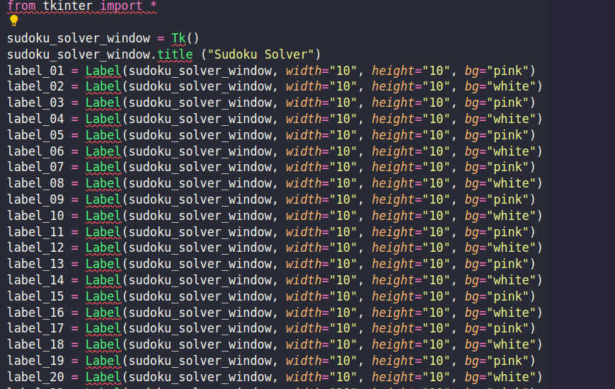
Excuse my Python. I did spend like half an hour on that, and then coded this instead:
from tkinter import *
sudoku_solver_window = Tk()
sudoku_solver_window.title ("Sudoku Solver")
w = []
for k in range(81):
    i=int(k/9)
    j=int(k%9)
    if (j + i) % 2:
        w.append(Label(sudoku_solver_window, bg="pink", width=5, height=5))
    else:
        w.append(Label(sudoku_solver_window, bg="white", width=5, height=5))
    w[k].grid(row=i, column=j, padx=2, pady=2, ipadx=5, ipady=5)

mainloop()
Yeah, dictionaries are a life-saver. For SEO: Python dictionaries for creating variables through the power of for-loops.
New Update: This sudoku GUI is cute-and-all, but I came across the cutest most fantastic looking web-app for sudoku solvers: Sudoku with 4 digits by Aad van de Wetering.
Step 1.5: Making a Web-Based Application instead
To do this, I shall need to learn Javascript from scratch. The goal is to create a webpage that takes the input from user as a imgur image url/file and solve the puzzle to display the output on a grid that looks nice.
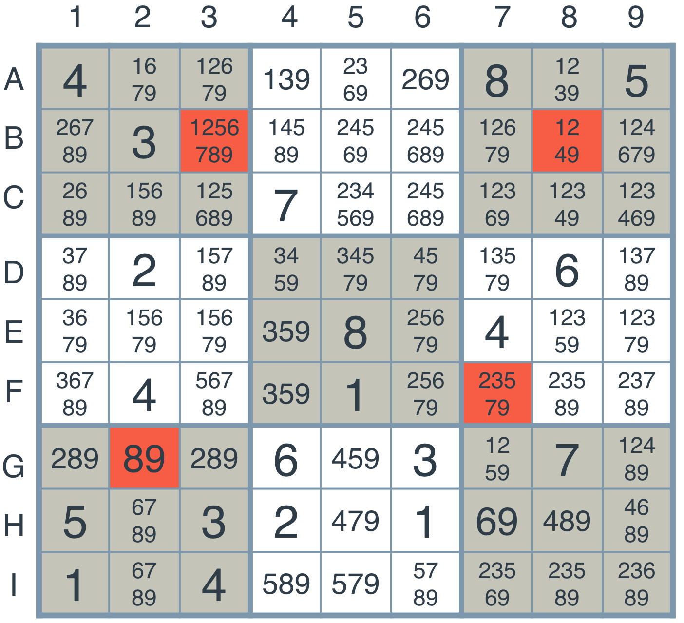
(Scroll your mouse over this grid, it’s fun)
| 1 | 2 | 3 | 4 | 5 | 6 | 7 | 8 | 9 |
| 10 | 11 | 12 | 13 | 14 | 15 | 16 | 17 | 18 |
| 19 | 20 | 21 | 22 | 23 | 24 | 25 | 26 | 27 |
| 28 | 29 | 30 | 31 | 32 | 33 | 34 | 35 | 36 |
| 37 | 38 | 39 | 40 | 41 | 42 | 43 | 44 | 45 |
| 46 | 47 | 48 | 49 | 50 | 51 | 52 | 53 | 54 |
| 55 | 56 | 57 | 58 | 59 | 60 | 61 | 62 | 63 |
| 64 | 65 | 66 | 67 | 68 | 69 | 70 | 71 | 72 |
| 73 | 74 | 75 | 76 | 77 | 78 | 79 | 80 | 81 |
Update: Instead of Javascript we’re probably going to figure out Brython: Python for Browsers. I’m having problems with the brython files, will return to it after building the machine learning model.
Update 2: No one uses Brython. I’m going to create a flask application instead.
Step 2: Extracting Text from Sudoku Puzzles
This step is also divided into two other steps. The first is essentially splitting the picture to digits and the second would be recognizing handwritten digits. The learning begins:
If you want to follow along with what I actually learnt visit this. I’ll give myself 2 more days and after a better understanding of the MNIST classification problem, we start to work towards the actual problem.
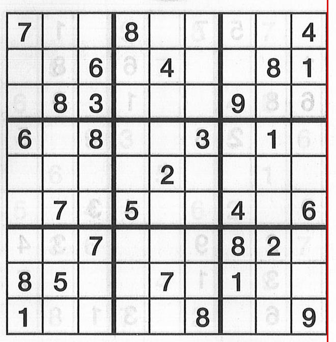
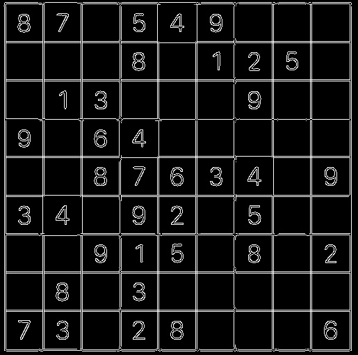
The next step is working with the actual sudoku image. Here, I’d like to introduce opencv’s most famous sudoku puzzle, dave.jpg.

I sat down to write the code, or copy-paste it from the website. It didn’t work out for me as well as it did for Dave.
For a really long time it was like only the vertical lines were being detected, so I thought maybe we could rotate the image and pass back into the function. I ended up with this monstrosity.

Ooof Madone! Have we created a masterpiece.
I tried a couple of more techniques and then read the old docmentation on hough lines. In this you come across several parameters one of which is a threshold:
HoughLines(dst, lines, 1, CV_PI/180, 150, 0, 0 );It is currently set to 150, what you want to do is play with it and tweak it to 160. So, from my understanding of that number is it sort of constrains you depending on how shitty the image you’re working with is. I could let the user decide but I also know lots of other projects deal with whatever image is thrown at them. Because I don’t want this project to go on forever and for the sake of my own sanity you can deal with cropped images from www.sudoku.com which is accessible by the user or really nice images like this one below, which I have a folder of.
def hougher(img):
    image1 = img
    gray=cv2.cvtColor(image1,cv2.COLOR_BGR2GRAY)
    dst = cv2.Canny(gray, 50, 200)
    # change 100 to 200, so that diagonal isn't detected
    lines= cv2.HoughLines(dst, 1, math.pi/180.0, 160, np.array([]), 0, 0)
    a,b,c = lines.shape
    for i in range(a):
        rho = lines[i][0][0]
        theta = lines[i][0][1]
        a = math.cos(theta)
        b = math.sin(theta)
        x0, y0 = a*rho, b*rho
        pt1 = ( int(x0+1000*(-b)), int(y0+1000*(a)) )
        pt2 = ( int(x0-1000*(-b)), int(y0-1000*(a)) )
        cv2.line(image1, pt1, pt2, (0, 0, 255), 7, cv2.LINE_AA)
    cv2.imwrite('hough5.jpg',image1)
    return image1
And viola!
So there’s a fascinating bit of math behind hough transforms, this is my attempt to explain what is happening here. First your picture is converted to something that looks like this using an edge detection algorithm called Canny Edge Detection.
To get to this image first cv2.Canny performs a gaussian blur to smooth out the image and eliminate any noise. The way a gaussian blur works is we have two 2D matrices one is a kernel and the other of the image we have to work on. Depending on the task(sharpen, blur, outline, etc.)at hand, the kernel can have different values and is usually a much smaller matrix than the image. This kernel passes all over the image matrix and this is what happens
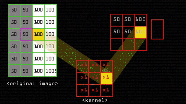
Original Image = \(A = \begin{bmatrix} 50_{0, 0} & 50_{0, 1} & 100_{0, 2}\\ 50_{1, 0} & 50_{1, 1} & 100_{1, 2}\\ 50_{2, 0} & 50_{2, 1} & 100_{2, 2}\\ 50_{3, 0} & 50_{3, 1} & 100_{3, 2}\\ 50_{4, 0} & 50_{4, 1} & 100_{4, 2}\\ \end{bmatrix}\)
Kernel for blur = \(K = \begin{bmatrix} 0.0625 & 0.125 & 0.0625\\ 0.125 & 0.25 & 0.125\\ 0.0625 & 0.125 & 0.0625\\ \end{bmatrix}\)
We select an element for the sake of an example let’s take it to be \(x_1, y_1\), now select all numbers surrounding it as well and you have this matrix:
Selected Portion = \(\begin{bmatrix} 50_{0, 0} & 50_{0, 1} & 100_{0, 2}\\ 50_{1, 0} & 50_{1, 1} & 100_{1, 2}\\ 50_{2, 0} & 50_{2, 1} & 100_{2, 2}\\ \end{bmatrix}\)
You multiply all of these values with the corresponding values of the kernel \(\begin{multline*}\\ 50\times0.0625 + 50\times0.125 +\\ 100\times0.0625 + 50\times0.125 +\\ 50\times0.25 + 100\times0.125 +\\ 50\times0.0625 + 50\times0.125 +\\ 100\times0.0625 = 218.5\end{multline*}\)
This is the convolution operation.
and then finally average it out: \(218.5/9 = 24.277777\)
I found a really neat blog to demonstrate this. To understand how kernels are calculated I recommend reading this.
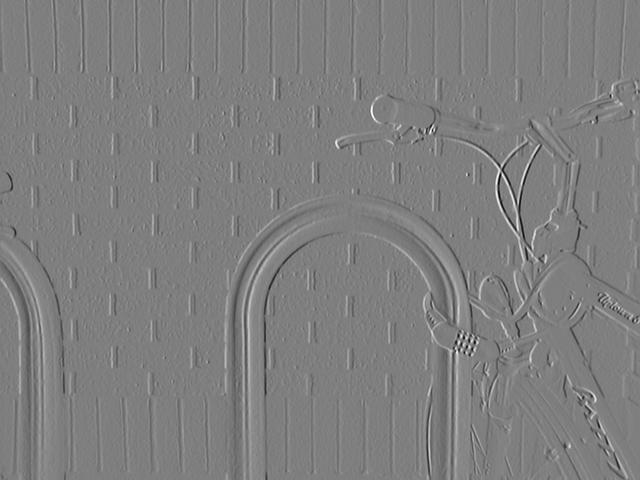
After smoothing the image and eliminating the noise, the next step is to find the edge strength by taking the gradient of the image. The Sobel operator performs a 2-D spatial gradient measurement on an image. Then, the approximate absolute gradient magnitude (edge strength) at each point can be found. The Sobel operator uses a pair of 3x3 convolution masks, one estimating the gradient in the x-direction (columns) and the other estimating the gradient in the y-direction (rows). These are:
\[G_x = \begin{bmatrix} -1 & 0 & +1\\ -2 & 0 & +2\\ -1 & 0 & +1\\ \end{bmatrix} * A\] \[G_y = \begin{bmatrix} +1 & +2 & +1\\ 0 & 0 & 0\\ -1 & -2 & +1\\ \end{bmatrix} * A\]where \(*\) represents here denotes the 2-dimensional signal processing convolution operation. This all is fine, but I want you to see the magic of this specific convolution in detecting edges.
\[\begin{bmatrix} 0 & 0 & 0 & 1 & 1 & 1\\ 0 & 0 & 0 & 1 & 1 & 1\\ 0 & 0 & 0 & 1 & 1 & 1\\ 0 & 0 & 0 & 1 & 1 & 1\\ 0 & 0 & 0 & 1 & 1 & 1\\ 0 & 0 & 0 & 1 & 1 & 1\\ \end{bmatrix} * \begin{bmatrix} -1 & 0 & +1\\ -2 & 0 & +2\\ -1 & 0 & +1\\ \end{bmatrix} = \begin{bmatrix} 0 & 4 & 4 & 0\\ 0 & 4 & 4 & 0\\ 0 & 4 & 4 & 0\\ 0 & 4 & 4 & 0\\ \end{bmatrix}\]Then you can proceed to apply a min-max scalar, convert the matrix to
\[\begin{bmatrix} 0 & 255 & 255 & 0\\ 0 & 255 & 255 & 0\\ 0 & 255 & 255 & 0\\ 0 & 255 & 255 & 0\\ \end{bmatrix}\]Identifying exactly where the color changes, where you can imagine 0 is black and 255 white.
In a similar manner, you can pass \(G_y\) which the horizontal Sobel filter to highlight the horizontal edges.
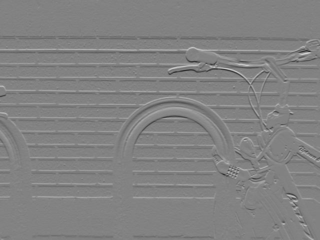
Then, you want both of them being represented together so you add up both the gradients \(G = \sqrt{G_x^2 + G_y^2}\). And similarly you could perform \(\theta = atan(\frac{G_y}{G_x})\) to the edge angle represented by different colors. This would look something like this:
Now the output of the sobel operator passes to the canny edge detector function. Canny takes the edges from sobel, suppresses the edges to show where the edges are located and not how wide are they. To do this canny checks what the orientation of the edge is and for all the neighbouring edges it has find which one form the local maximum.
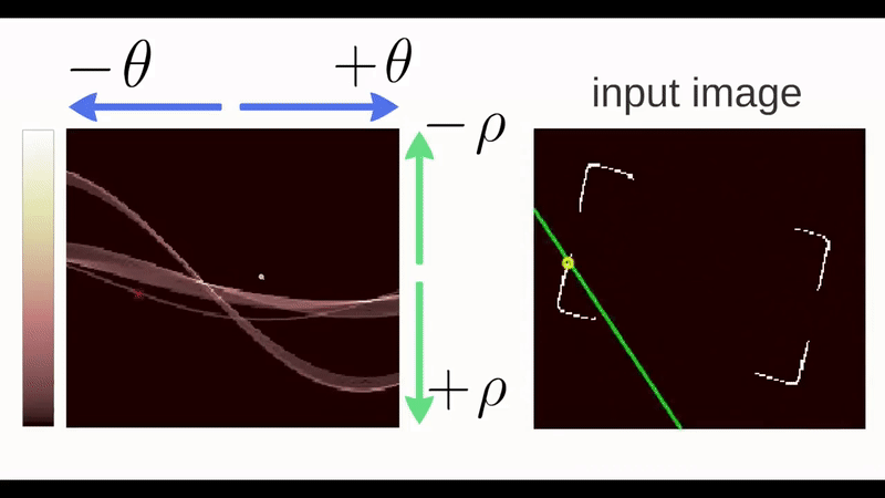
After this we perform a hough transform. Let’s try and break that down too.
This is the equation of a line:
If you pick two points \(x_i, y_i\) and \(x_j, y_j\) namely, they’d have the following equation: \(y_i = ax_i + b\) and \(y_j = ax_j + b\). Inverting these lines on plane \(a, b\) the equations become \(b = -x_i + y_i\) and \(b = -x_j + y_j\) then these lines would intersect at point \((a, b)\)

Another way to consider a line is through this eqaution: \(xcos\theta + y sin \theta = \rho\)

Any line can be represented in these two terms, \((\rho,\theta)\). So first it creates a 2D array or accumulator (to hold the values of the two parameters) and it is set to \(\theta\) initially. Let rows denote the \(\rho\) and columns denote the \(\theta\). Size of array depends on the accuracy you need. Suppose you want the accuracy of angles to be 1 degree, you will need 180 columns. For \(\rho\), the maximum distance possible is the diagonal length of the image. So taking one pixel accuracy, the number of rows can be the diagonal length of the image.
Consider a 100x100 image with a horizontal line at the middle. Take the first point of the line. You know its \((x,y)\) values. Now in the line equation, put the values \(\theta=0,1,2,....,180\) and check the \(\rho\) you get. For every \((\rho,\theta)\) pair, you increment value by one in our accumulator in its corresponding \((\rho,\theta)\) cells. Then keep doing this for all the points and if it finds corresponding points of edges they get highlighted in the first graph shown in the image below.
In addition to this, you can also watch this video by Thales Sehn Körting.
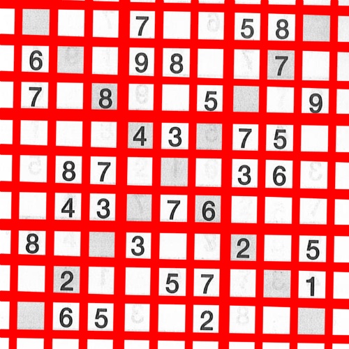
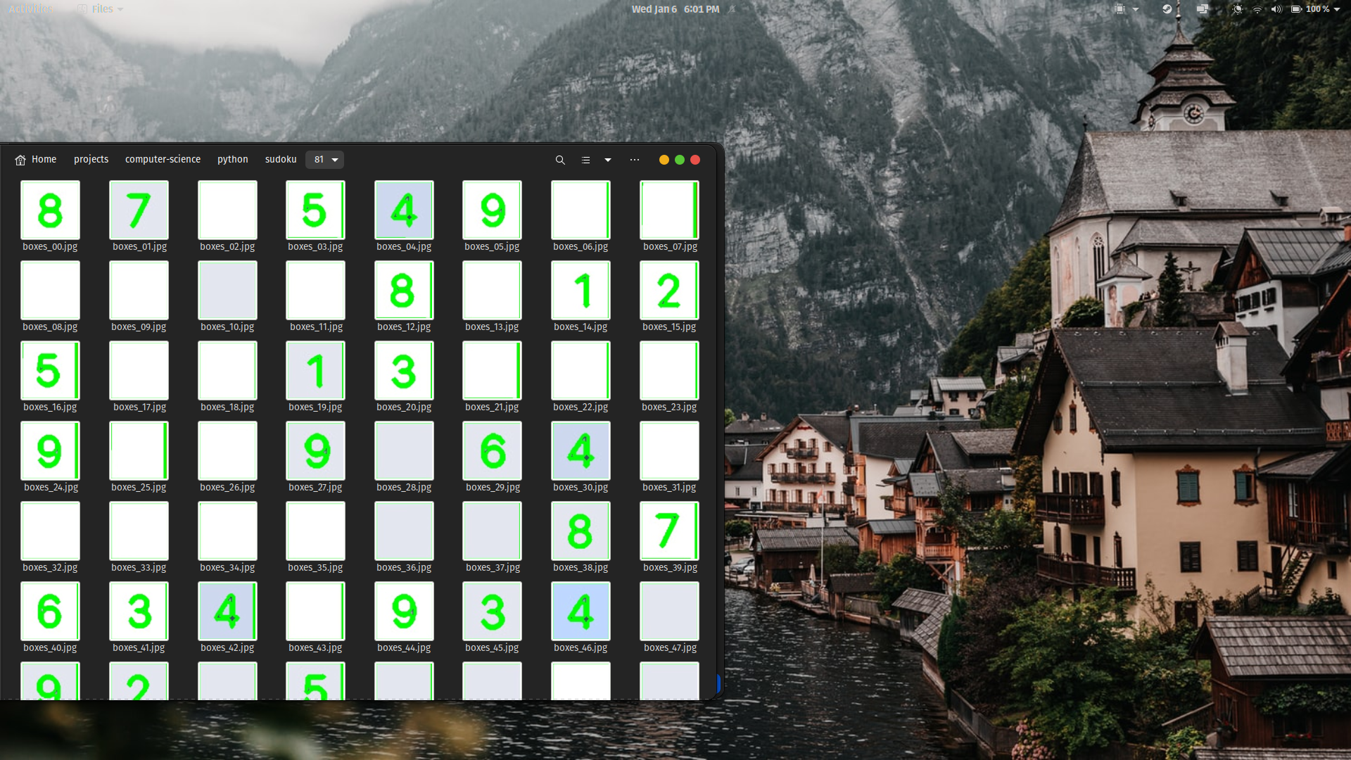
After the hough lines, I decided to contour draw contours on the image and extract 81 nice square images of digits.
def squares(img):
    gray = cv2.cvtColor(img, cv2.COLOR_BGR2GRAY)
    blur = cv2.medianBlur(gray, 5)
    sharpen_kernel = np.array([[-1,-1,-1], [-1,9,-1], [-1,-1,-1]])
    sharpen = cv2.filter2D(blur, -1, sharpen_kernel)

    thresh = cv2.threshold(sharpen,160,255, cv2.THRESH_BINARY_INV)[1]
    kernel = cv2.getStructuringElement(cv2.MORPH_RECT, (3,3))
    close = cv2.morphologyEx(thresh, cv2.MORPH_CLOSE, kernel, iterations=2)

    cnts = cv2.findContours(close, cv2.RETR_TREE, cv2.CHAIN_APPROX_SIMPLE)
    cnts = cnts[0] if len(cnts) == 2 else cnts[1]
    img = cv2.drawContours(img, cnts, -1, (0,255,0), 3)
    cv2.imwrite("con.jpg", img)
    min_area = 4000
    max_area = 11000
    image_number = 0
    # print (cnts)
    for c in cnts:
        area = cv2.contourArea(c)
        if area > min_area and area < max_area:
            x,y,w,h = cv2.boundingRect(c)
            ROI = img[y:y+h, x:x+h]
            cv2.imwrite('81/boxes_{}.jpg'.format(str(80-image_number).zfill(2)), ROI)
            cv2.rectangle(img, (x, y), (x + w, y + h), (36,255,12), 2)
            image_number += 1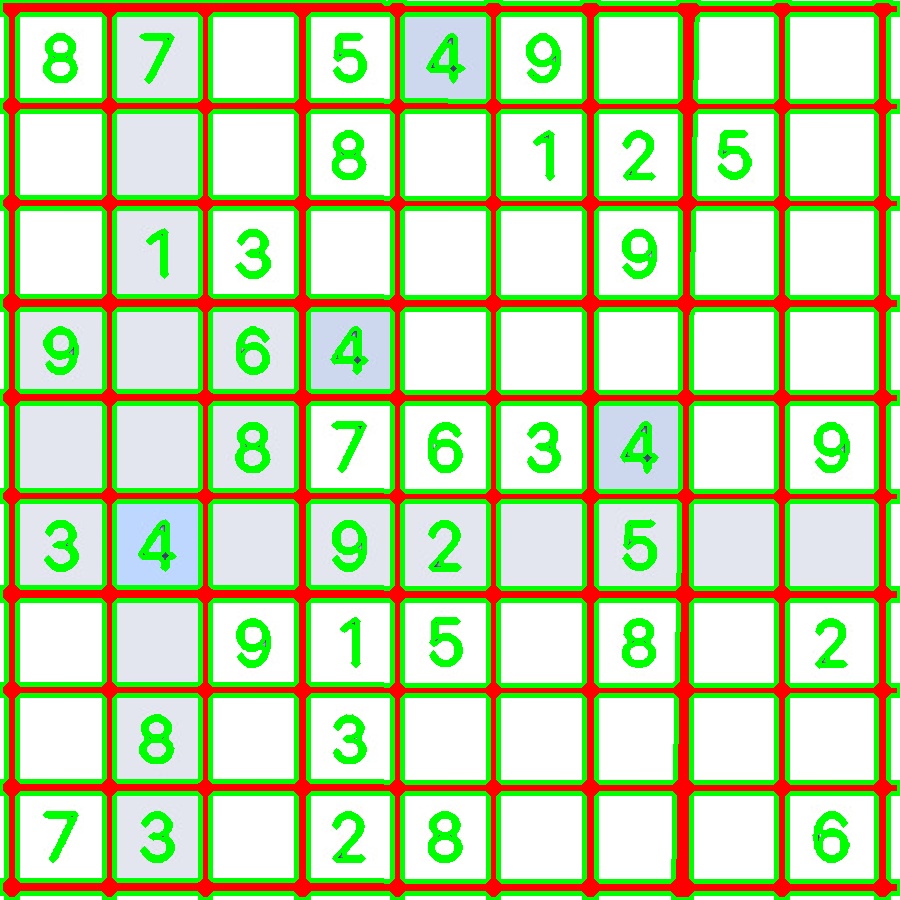
Then I sat down to train a model on the MNIST data using this video and
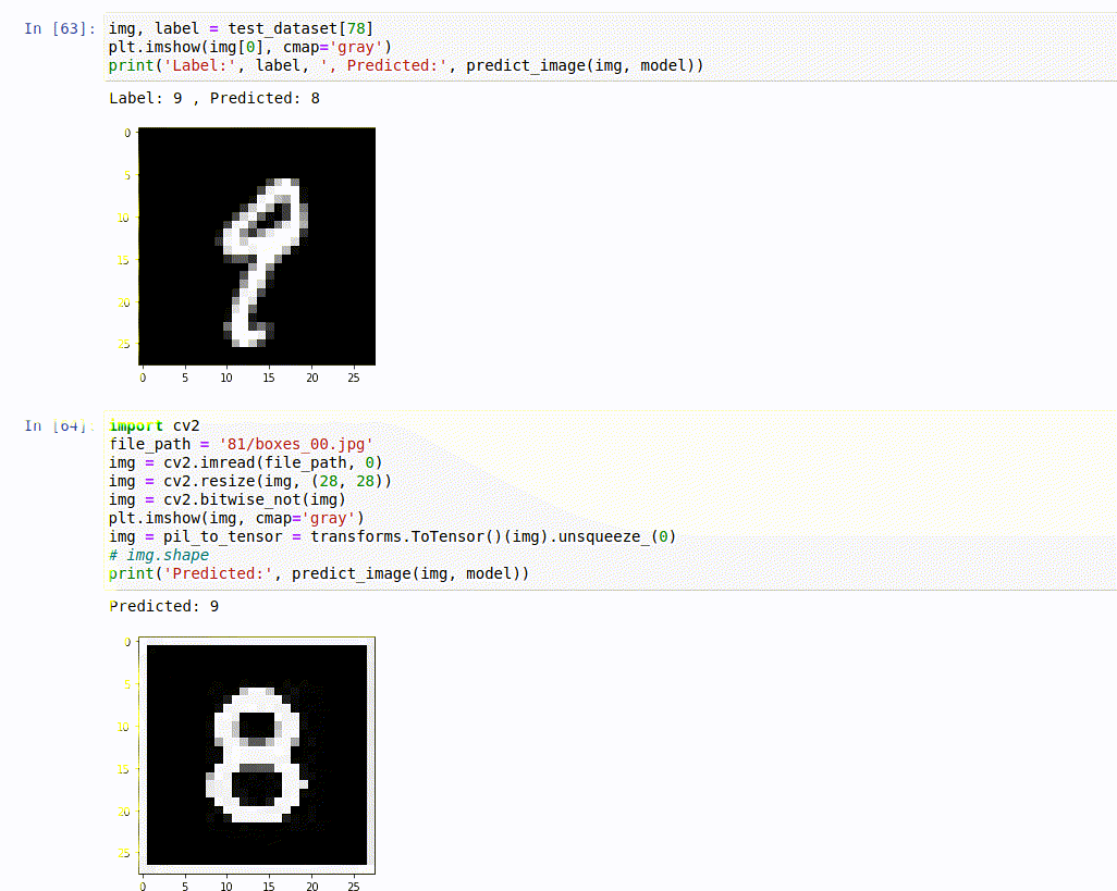
I don’t know if you can see it all too well, but that gif shows that MNIST can’t predict its own data correctly(at 98.64% accuracy), let alone mine. This just means, one mistake and it’s a wrong solution. At this point I took the world’s most boring decision, and decided to create my own dataset, so that at least we could get sudoku.com’s sudoku’s right. Although this model is a little flexible, but it would guarantee best results with the sudoku’s from there. And that’s how I cut 18 different puzzles with the power of laser technology to create my very own… you get the point. After collection I sat down to train a model using Youtube videos from Sentdex and have definitely had my fair-share of keras, numpy, reshaping and CNNs.
model = Sequential()
model.add(Conv2D(64, (5,5), input_shape = X.shape[1:]))
model.add(Activation("relu"))
model.add(MaxPooling2D(pool_size=(2,2)))

model.add(Conv2D(64, (5, 5)))
model.add(Activation('relu'))
model.add(MaxPooling2D(pool_size=(2, 2)))

model.add(Flatten())  # this converts our 3D feature maps to 1D feature vectors
model.add(Dense(64))

model.add(Dense(32))
model.add(Activation('relu'))

model.add(Dense(16))
model.add(Activation('relu'))

model.add(Dense(10))
model.add(Activation('softmax'))

model.compile(loss='sparse_categorical_crossentropy',
              optimizer='adam',
              metrics=['accuracy'])

model.fit(X, y, batch_size=256, epochs=25, validation_split=0.3)
I must say, it paid off pretty well. 100% accuracy. Not just because the model says so, but I’ve seen it with my own two eyes. As far as I go, I can’t claim the 100 so I’ll say 98.64% too, for whenever things go south.
Yeah, I’m going to break down this code as well, but this time it’ll be short I promise. Like before we’re processing image pixels and the first step is performing a convolution on them to create feature maps of them. Then max-pooling helps us select the maximum value in that region which then becomes the value for the entire region in that image.
Most classification code looks like some form of this one. Depending on the problem really just few of these numbers and variables change, but that change is significant. In this particular case we wanted to perform a multi-class classification such that every picture that’s told to be predicted through this network can have just one class as its predicted. To ensure such is the case that last layer is a softmax and we perform a categorical crossentropy. I’d recommend reading this.
Step 3. We Solve the Puzzle
We have options here, like a lot of good options and some bad ones too. Let’s iterate through them.
- The shortest sudoku solver by David Singleton. Find out more here.
class S{public static void main(String...a){int i=a[0].indexOf(48),j;char
k=48,c[]=a[0].toCharArray();if(i<0)System.out.print(c);else
for(;++k<58;){for(j=81;j-->0&&((j-i)%9*(j/9^i/9)*(j/27^i/27|j%9/3^i%9/3)
|c[j]^k)!=0;);c[i]=k;if(j<0)main("".valueOf(c));}}}
It’s a shame he uses Java, he could’ve bagged the ioccc with this stuff. We’re not going to be using this, because the title says ML and the solutions given out by this algorithm were a little off.
- The backtracking AI sudoku solver.
Here the rules are expilicitly being coded, which is not something meant by machine learning. Instead of showing you the code, I’ll instead
![]()
Yes, can you see see how many numbers are changing in one frame. If you can then, well done Usain Bolt of vision. So, if AI is supposed to mimic human intelligence, do humans really backtrack at the scale? I would imagine most normal humans doing something like this:
 and that is how we come to
- Peter Norvig’s Solution
[draft]
- The most horrifying RNN.
Now generally I don’t think stuffing everything with a network is required. Quite the contrary. I hate AI, ML and object oriented programming, call them over-exploited buzzwords. Unrelated to this, but I came across this blog post, where Joel Grus thinks it fit to solve a fizzbuzz problem with a convnet. Thing is, it got some of the answers wrong, it’s not fast, and just in general a stupid thing to do. When this translates to the sudoku problem, it gets kind of crazy.
If a convnet can’t predict the answer for fizzbuzz, getting 81 numbers right in row is kind of like the time Bach’s work was described as playing 6 games of chess blindfolded and still winning. Which got me wondering about this. How many iterations of input and output strings of unsolved sudokus and their respective solutions would it take for a computer to realize a pattern in the data. Certain obvious ones like the numbers used only range from 1 through 9 and lesser obvious ones like all the rules for playing. And consecutively, how long till a person who has never heard of sudokus to realize this. I obviously don’t have a batch of people to test this on but…
I decided to create a hybrid RNN. One that guesses one number at a time(like humans) knows the rules and still is trained on a set of 1 million games of sudoku. The most inefficient and long solution. I’m only doing it for the title, and because backtracking seems morally wrong.
Update: It’s January 13th and I’ve been considering using NLP to solve them at this point. However, I’ve come to a major decision. This neural network is fundamentally going to be different. Now, traditional ones create their own perception of things. Like the model we made for guessing the numbers isn’t so because we said that the pixel at x,y has to be black then it’s a 1. But something like sudoku does have these rules embedded in it. You can’t place a number where it’s not meant to be, because the model predicted it. For this we’re going to be constructing constraint masks instead. Constraint masks are a cheat too in some way.
The other way of looking at this problem is not considering it so much of a processing problem but looking at it as generating problem first. It’s like teaching a kid English. You first let him speak his mind and correct him wherever you feel the grammar is wrong. After a while he’s generating correct sentences and the to test him you give him a blank to fill in, in a sentence.To even better it, the kid now has to deal with two blanks in sentence where one blank’s value depends on the other. In this case, the child must be able to go to a previuos blank so as to make the sentence grammatically correct. [draft: Bluert, NLG, LSTMs with Attention]
It’s February 6th, and I’ve come up with yet another way to think of games. I have two examples: have you seen one of those ML videos where they teach the code to learn something like Mario Kart and it works on a feedback loop, so in every iteration it’s looking to be better by getting feedback on the move it makes. We could just apply that to our algorithm and what would happen is, as tries to fill something and subsquently knows the answer of, we create a feedback loop. The other example is of yo-yos. The unspoken rule of a yo-yo is that has to come back in your hand. Even if someone hasn’t explicitly told that to you that rule you just start to have an intuition. This probably refers to a more abstract and tactile based intuition, but what I’m concerned with now is how do we begin to harbor such.
I do think I’ll have to write a part 2 of this blog post to cover the techanicalities of solving such problems.
Step 4: Back to the Website
I started working with Flask at first and for reasons unknown I couldn’t get the GET and POST requests to work. If you would want to try watching DeepLizard’s series and if you don’t want to waste more time get started with Django. To setup your web aplication watch this guide and really half way through it you’ll start to get an intuition of how Django works. By the end for designing the front-end you’ll need some knowledge on the built-in tags which if you’ve ever worked with Liquid you’ll get a hang of pretty easily.
After I was done with building the web-app I lost my head on deploying it. You can’t use plain vanilla Heroku deployment because for some stupid reason they decided on not supporting python libraries like scipy, scikit and whatnot. The solution they list out is then using Docker and try following this video by VeryAcademy. Now Docker is a real pain in the ass, it’s one script that takes an hour to run and the whole time your fingers are crossed like pretzels hoping not to run into errors. Protip: Do not use Alpine. and better yet just copy paste my Dockerfile. I’ve literally wasted days on this… when Dockerfiles could’ve simply been venvs with single commands being run at a time because forging for every dependency before an install is a nightmare.
Resources:
-
The Augmented Reality Sudoku Solver by atomic14: I listened to this video line-for-line and still don’t get how he does the very first step. But, to get started it’s fine. Also, his project is pretty damn good.
-
Another Sudoku Solver by Murtaza’s Workshop: Went through this half-way and it didn’t work out but my project is somewhat more similar to his (and pssst… it’s much shorter).
-
Zero to GANs on Jovian: Understanding MNIST and the basics of ML and why it screwed couple of my days here on earth. But yeah, the guy who teaches the course absolutely amazing, you should definitely take the course.
-
Classification Problems by Sentdex: I think Sentdex is god-sent, he’s like the Bucky Roberts of ML (and after doing this I’m like the Siraj😂).
-
The amazing documentations of Pytorch, OpenCV, Django, Docker, NGINX and of course Stackoverflow.
My Code
Visit: Sudoku Solver:v1
Unrelated Gems I came across:
-
The Soparanos is a great show.
-
Songs that can help you cope: Strange Powers by the Magnetic Fields, Self Portrait by Matty, and I recently found out Arpeggi by Kelly Lee Owens is actually stripped from Thom Yorke and it’s uhm… great without him.
-
Since we’re already off to a weird tangent and I’ve spewed 3000 words on sudokus, I know no one cares about them right. But something about bringing this up as random conversation always gets sparks everywhere and I hoped you enjoyed reading.