Reinforcement Learning based Sudoku Players, Part 2

After about a month of learning deep learning, I realized the solution to the sudoku problem after coming across one single word: Gridworld.

Another square matrix like sudoku, that looks like this:

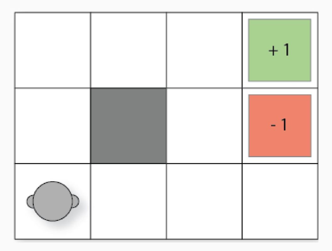
Now to solve the Gridworld problem through machine learning you require a special system, a fancy word: Deep Q-networks.

I write this as I embark on a journey to solve it myslf, so writing is what helps me jot down ideas and teach myself.

Deep Q-networks is quite novel, in the sense that we don’t have too many videos tutorials. I don’t think many of us actually want to read probability equations from Sutton’s book. To get a basic idea I recommend watching Jabrah Tutorials series on Reinforcement Learning.

After that we’re going to quickly run through all these terms to model this infrastructure to our own needs.

Bet you’ve heard of a markov chain…

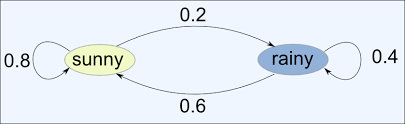
If you haven’t then it’s really simple. This one basically just says this:

If sunny today, then tommorow: 80% probability for sunny 20% probability for rainy

If rainy today, then tomorrow: 60% probability for sunny 40% probability for rainy

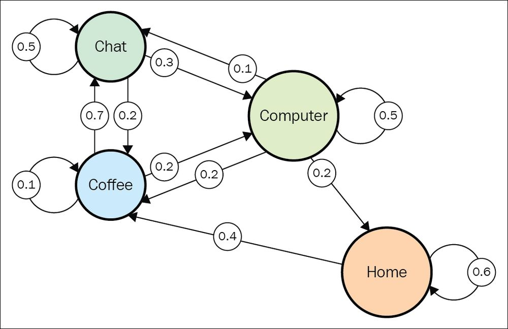
If you were to make a markov chain of your life it would be somthing like this:

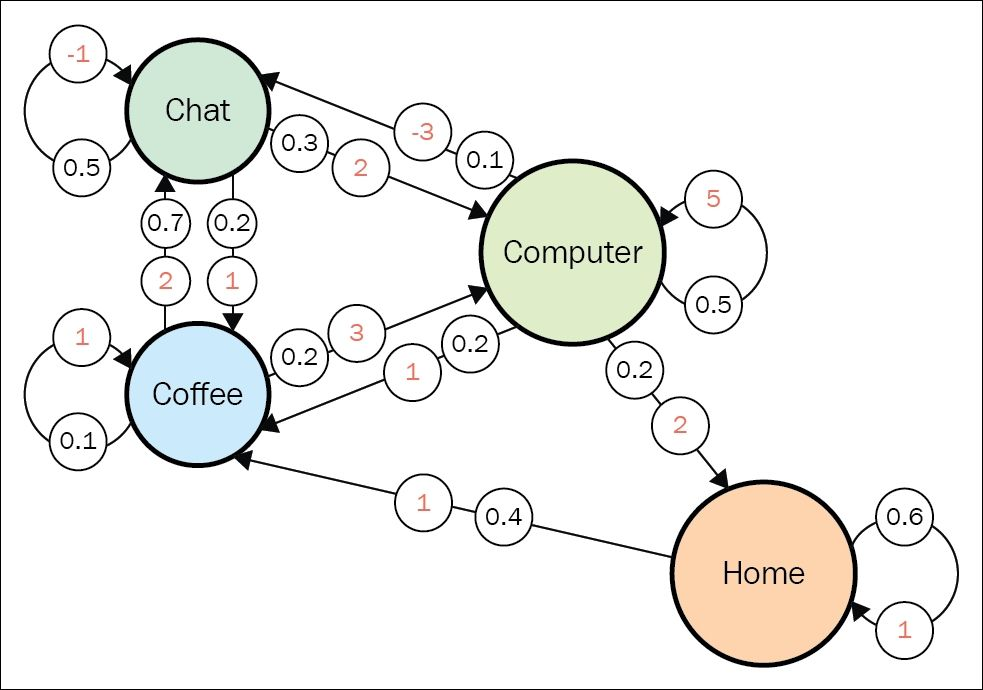
Now these are just the probablities of taking an action, I want to add another dimension to it. Say if we were to reward a task, negatively if the task is bad for the person’s productivity and positively if it is good. The agent in such a markov chain wants to perform better, he’s a motivated guy that loves getting rewards.

Some important terms

Any time we observe the system we are recording an episode. For example here it could be home → coffee → coffee → chat → chat → coffee → computer → computer → home. Wherein each of the different tasks are states the agent could be in.

The other thing to note down here is that the transition distribution for any state doesn’t change over time. Non-stationarity means that there is some hidden factor that influences our system dynamics, and this factor is not included in observations.

Now we understand actions. Our agent at every step has a set of action \((A)\) which is finite. This is our agent’s action space. For this we add another dimension, making it a cube with the transition matrix. Now the agent no longer passively observes state transitions, but can actively choose an action to take at every time. So, for every state, we don’t have a list of numbers, but a matrix, where the depth dimension contains actions that the agent can take, and the other dimension is that the target state system will jump to after this action is performed by the agent.

When we talk about taking an action in a particular state we call it a state-action pair \((s, a)\).

Now the agent doesn’t observe transitions passively but instead can take actions and affect the probabilities of the target states.

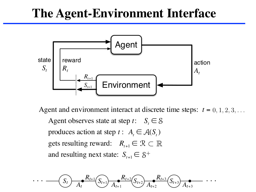
If an RL task has a Markov properties it is a Markov Decision Process. If the state and action sets are finite we have a finite MDP. To define a finite MDP we have one step dynamics: \(p(s', r|s, a) = Pr(S_{t+1}= s', R_{t+1}=r|S_t=s, A_t=a)\). This is the probability of being in state \(s'\) and receiving reward \(r\) after being in state \(s\) and performing action \(a\).

A policy defines how an agent acts from a specific state. For a deterministic policy, it is the action taken at a specific state. RL defines how the agent needs to change its policy as a result of experience, and here generally the goal is to maximise the rewards. However there could be a variety of policies: like go haywire, avoid just the obstacles, or spin around.

Policy at step \(t = \pi_{t} =\) a mapping from states to action probabilities \(\pi_{t}(a|s) =\) probability that \(A_t = a\) when \(S_t = s\).

Deterministic policies are \(\pi_t(s) =\) the action taken with probability = 1 when \(S_t = s\).

Now the sequence of rewards after step \(t\) is: \(R_{t+1}, R_{t+2}, R_{t+3}, ...\)

Here we seek to maximise:

• Total Reward, \(G_t = R_{t+1} + R_{t+2} + R_{t+3} + ... + R_T\). This is usually taken in episodic tasks like number of times the game was played, and we just add the sum total of all the rewards.
• Discounted Reward, \(G_t = R_{t+1} + \gamma R_{t+2} + \gamma^2 R_{t+3} + ...\\= \sum_{k=1}^{\infty} \gamma^k R_{t+k+1}\)This is taken for continuing tasks, where there aren’t just episodes that come to an end but at every consecutive action it is required to avoid failure. Here \(\gamma, 0 <= \gamma <= 1\). If \(\gamma\) tends to zero this that means the agent is short-sighted, whereas if it tends to 1 it is farsighted. Generally, we take \(\gamma = 0.9\) because we need to discount the current rewards so that the agent performs better in the whole. If \(\gamma = 1\) then the value is infinite for all states. And if our diagram doesn’t have any sink states(states without any outgoing transitions) then we’re looking at an infinite amount of transitions. When \(\gamma = 0\), all our values are positive in the short term and so the infinite sum of positive values will give us an infinite value regardless of the starting state. This infinite result shows us one of the reasons to introduce gamma into a Markov reward process, instead of just summing all future rewards. In most cases, the process can have an infinite (or large) amount of transitions. As it is not very practical to deal with infinite values, we would like to limit the horizon we calculate values for. Gamma with a value less than 1 provides such a limitation. We can have \(\gamma = 1\) in a tic-tac-toe game where there is a sink state after just 9 turns of playing.
• Average Reward, \(G_t =\) average rewards per time step. This mean shall be measured by \(\mu = 1/k \sum_{k=1}^{k} R_{t+k+1}\) but to consecutively update the mean we use: \(\mu_{new} = (k.\mu_{old} + R_{t}) / k + 1\).

Let’s understand with an example: The Mountain Car example.

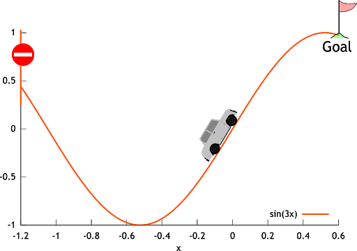
The goal is to get to the top of the hill as fast as possible. Here, reward = -1 for each step we aren’t at the top of the hill and so \(=>\)return = -number of steps before reaching the top of the hill.

Now, we are going to understand how to calculate the value of state. Denoted by \(V(s)\), this value function measures potential future rewards we may get from being in this state \(s\).

For this the values of each state is:

\(V(coffee) = 2 * 0.7 + 1 * 0.1 + 3 * 0.2 = 2.1\) \(V(chat) = -1 * 0.5 + 2 * 0.3 + 1 * 0.2 = 0.3\) \(V(home) = 1 * 0.6 + 1 * 0.4 = 1.0\) \(V(computer) = 5 * 0.5 + (-3) * 0.1 + 1 * 0.2 + 2 * 0.2 = 2.8\)

Just take a state and then look at all the arrows heading out of that state, multiply the rewards and probability and then perform the summation for all the outgoing transitions.

OpenAI Gym and the anatomy of an agent…

Let’s setup a basic program:

class Environment:
	def __init(self):
		self.steps_left = 10
		# initializing env by saying that only 10 steps are left

	def get_observations(self):
		return [0.0, 0.0, 0.0]
		# returns the current envs observation to agent
		# it's some function of the internal state of the env
		# here the observation vector is always zero because the env has no internal state

	def get_actions(self):
		return [0, 1]
		# set of actions the agent can perform
		# usually this doesn't change over time
		# but smetimes certain moves aren't possible

	def is_done():
		return self.steps_left == 0
		# check if episode is completed

	def action(self):
		if self.is_done():
			raise Exception("Game is Over")
		self.steps_left -= 1
		return random.random()
		# if episode is completed then raise exception
		# else just take an action and subtract a step from step_left.

class Agent:
	def __init__(self):
		self.total_reward = 0.0

	def step(self, env):
		current_obs = env.get_observation()
		# observe env
		actions = env.get_actions()
		# make a decision of action to take
		reward = env.action(random.choice(actions))
		# submit action and collect the rewards
		self.total_reward += reward

if __name__ == "__main__":
	env = Environment()
	agent = Agent()

	while not env.is_done():
		agent.step(env)
	print("Total reward got: %.4f" % agent.total_reward)

This piece of code is important as it is the infrastructure of our RL agent.

OpenAI provides us with the environment: set of actions, observations, method called <div class="inlinecode">step</div> to execute an action (returns current observation, reward, and indication that the episode is over), a method called <div class="inlinecode">reset</div> to retrun to initial state.

https://jonathan-hui.medium.com/rl-reinforcement-learning-terms-242baac11907

http://incompleteideas.net/book/first/ebook/node34.html